Darwin Meets Graph Theory on a Strange Planet: Counting Full \(n\)-ary Trees with Labeled Leafs

Johnathan Barnett and Hannah Correia

Huntingdon College

Peter Johnson, Michael Laughlin, and Kathryn Wilson

Auburn University

Introduction

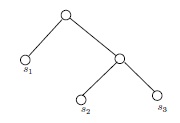
Some time in April 2009, the third author ran across some numbers in Chapter 10 of The Blind Watchmaker (Dawkins, 1996), a popular explanation of evolution by the great evolution explainer Richard Dawkins, that he (the third author) could not verify. These numbers were counts of different ``family trees'' indicating degrees of ``cousinhood'' or order of descent, among categories of living things. For example, if we are interested in (relative) cousinly relations among 3 species, say lions and tigers and bears (assuming those to be species), there are 3 hypothetical trees to consider:

(Please understand that, for instance, is the same as the last of the 3 trees above.)

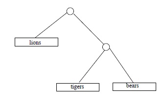
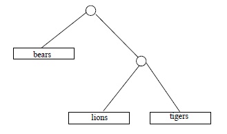
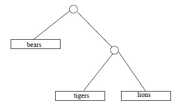
Dawkins casually asserts that with 4 species there are 15 different family trees; with 11 species, 654,729,075 possible trees; and with 20 species, the number of different possible trees is 8,200,794,532,637,891,559,375, according to Richard Dawkins.

The third author puzzled over these figures for a bit, hoping to discover the formula or process by which they were obtained. No inspiration bloomed; the question was stowed in a special file for possible future use in Auburn University's Research Experience for Undergraduates in Algebra and Discrete Mathematics. Fifteen months later the file was opened and the question answered. This led to a harder question, which was also answered, to the amazement of the third author; the coup de grace was administered months after the end of our 2010 REU by the second author, with the assistance of the first. What follows is an account of the results discovered. These discoveries are not new (although one proof might be), but that does not mean that they are widely known. At the least, our inquiry involves the resurrection of a great nineteenth century theorem in graph theory.

Definitions and fundamentals

A graph is a very simple geometric object, a pair of sets \((V, E)\), in which \(V\) is the set of vertices, or nodes, and \(E\) is the set of edges. The only geometric assumption is that each edge has two ends, and at each end is a vertex of the graph. If \(v \in V\) is at one end of \(e \in E\), we can say that that end of \(e\) is sticking into, or incident to, \(v\). The two vertices at the ends of an edge are said to be adjacent in the graph.

If both ends of \(e \in E\) are incident to the same \(v \in V\), we say that \(e\) is a loop. If \(v, w \in V\) are the two vertices at the ends of two or more different edges of the graph, then we say that \(vw\) is a multiple edge of the graph. If a graph has no loops nor multiple edges, it is simple.

Figure 1: A graph with a loop and a multiple edge, and a simple graph

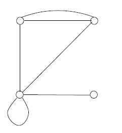
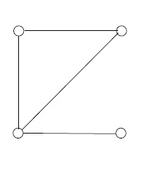
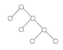
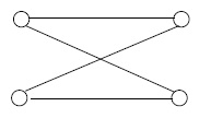
For any graph \((V, E)\), the degree, or valence , of a vertex \(v \in V\) is the number of edge ends sticking into it. For example, in Figure 1, above, there are vertices of degrees 3, 3, 5, and 1 in the non-simple graph, and vertices of degrees 2, 2, 3, and 1 in the simple graph. There is a fundamental numerical relation between the degrees and the number of edges in any finite graph: the sum of the degrees is twice the number of edges. This fact, which comes in quite handy, arises from the requirement that each edge has two ends, and so is counted twice in taking the sum of the degrees.

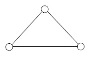
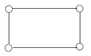
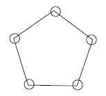
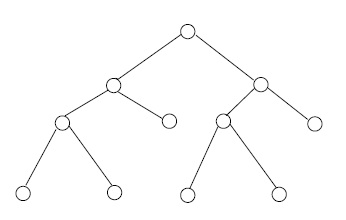
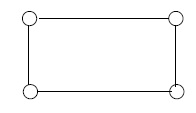
A graph is connected if a bug can walk from any vertex of the graph to any other vertex along the edges of the graph. For \(n \geq 3\) the cycle \(C_n\) is the graph that can be drawn to look like a regular polygon with \(n\) vertices and \(n\) sides. See Figure 2.

Figure 2: \(C_3\), \(C_4\), and \(C_5\)

A simple graph is acyclic if it contains no \(C_n\), \(n \geq 3\), as a subgraph. A tree is an acyclic connected simple graph. The one fact about trees that we shall need is this: in every finite tree, the number of edges is one less than the number of vertices. Therefore, in a tree on \(p\) vertices, the degree sum is \(2p-2\).

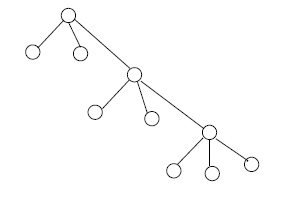
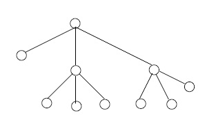
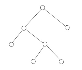
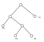
For an integer \(n \geq 2\), a full \(n\)-ary tree is a finite tree with one vertex, the root, of degree \(n\), and with all other vertices of degrees 1 or \(n + 1\). In the cases \( n = 2, 3 \) we write binary, ternary rather than 2-ary, 3-ary, respectively. The vertices of degree 1 in any tree are called leafs. See Figure 3.

Figure 3: Two full binary trees with 4 and 6 leafs, and two full ternary trees with 7 leafs each.

Suppose that \( G \) is a full \( n \) -ary tree with \( m \) leafs and \(k\) non-leafs. By a previous remark about degree sums in trees, we have \[ m + n + (k-1)(n+1) = 2(m+k) - 2,\] which implies \[m = (n-1) k+ 1.\] Therefore \(G\) has \(m + k = nk + 1\) vertices, and \(nk\) edges.

Suppose that \(G\) and \(H\) are simple graphs. An isomorphism from \(G\) to \(H\) is a function \(\varphi : V(G) \to V(H)\), one-to-one and onto, such that \(u, v \in V(G)\) are adjacent in \(G\) (i.e., \(uv \in E(G)\), in common notation) if and only if \(\varphi (u), \varphi(v)\) are adjacent in \(H\). If there is an isomorphism \(\varphi\) from \(G\) to \(H\) then \(\varphi^{-1}\) is an isomorphism from \(H\) to \(G\); we say that \(G\) and \(H\) are isomorphic.

You can think of an isomorphism as moving the vertices of one graph onto the vertices of another graph and dressing the edges so that the "moved" graph coincides with the "target" graph. Thus two simple graphs are isomorphic if and only if they are (different) incarnations, or drawings, or representatives, of the same thing---their isomorphism class. This is by way of saying that "being isomorphic" is an equivalence relation on the set of (all drawings of) simple graphs. As in other areas of mathematics, it is customary to be casual about distinguishing between an isomorphism class and any particular representative of that class. Unless otherwise specified, the term graph henceforward will refer to an isomorphism class of simple graphs. See Figure 4.

Figure 4: Two different drawings of \(C_4\), and two different drawings of the same fulll binary tree.

Suppose that \(G\) and \(H\) are (representatives of) graphs and that in each there are \(m\) vertices distinguished by the same labels, \(s_1, \ldots, s_m\). We will say that \(G\) and \(H\) are isomorphic as partially labeled simple graphs if and only if there is an isomorphism from \(G\) to \(H\) which takes the vertex labeled \(s_i\) in \(G\) to the vertex labeled \(s_i\) in \(H\) for each \(i = 1, \ldots, m\).

Figure 5: Four full binary trees with labeled leafs. The top two and only the top two are isomorphic.

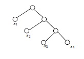
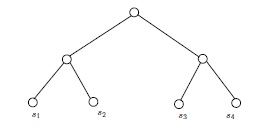
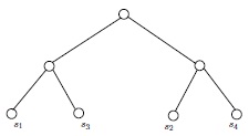
If \(G\) and \(H\) are isomorphic as partially labeled graphs, then they are isomorphic. Therefore, in Figure 5, the two (isomorphic) partially labeled trees on top cannot be isomorphic as partially labeled trees to either of the partially labeled trees below them. The two lower trees are clearly isomorphic as simple graphs, but not as partially labeled simple graphs. For one thing, the vertices labeled \(s_1\) and \(s_2\) have a common neighbor in one of the drawings, but not in the other.

Now we can make precise the problem sketched in the Introduction. The problem is to calculate the number \(f(m)\) of isomorphism classes of full binary trees with \(m\) leafs, labeled \(s_1, \ldots, s_m\).

It will seem obvious to many readers that these different isomorphism classes do indeed represent the different possible relative kinship relations or orders of descent among any \(m\) species, but even for those who are quite sure that they have grasped the connection between our mathematical counting problem and Dawkins' genealogical counting problem, it may prove useful to list some of the assumptions and premises involved.

1. Speciation is assumed to be binary, meaning that new species are formed by old species splitting into two. When this occurs in nature, usually one of the two ``new'' species is indistinguishable from the ``old'' {\em parent} species; nonetheless, in any modelling of species relations, the parent species will be considered to be distinct from each of its sibling children.
2. In a full binary tree with labeled leafs, representing a conjecture abut the order of descent of given species corresponding to the leaf labels, every node represents a (hypothetical) species. When two nodes are the sibling offspring of a parent node in the tree, it does not necessarily mean that the species represented by the parent node split into the two species represented by the sibling offspring nodes, although that is a possibility; rather, it means that the species of the parent node is a common ancestor of the two species of the sibling nodes, and not just any common ancestor, but the nearest common ancestor of the two. (We leave to the reader the pleasure of making precise what this means, and of verifying that any two species with a common ancestor have a unique nearest common ancestor.) For example, the tree would be Dawkins-interpretable as asserting that \(s_2\) and \(s_3\) have a common ancestor distinct from each, and that their nearest common ancestor has a common ancestor with \(s_i\); further, \(s_1\) is not the nearest common ancestor of \(s_2\) and \(s_3\), nor is \(s_1\) an ancestor of that nearest common ancestor.
3. From 2 it can be seen that the species represented by the labels on the leafs of a full binary tree purporting to depict the relative relatedness of them all must (if the depiction is correct) have a common ancestor, the root of the tree, and have no offspring species themselves---it would be said that these species are terminal. These necessary conditions on the cohort of species under consideration for there to be a valid depiction of their relatedness by one of our labeled trees are generally assumed uncritically. It behooves us to point out that these assumptions could, plausibly, be invalid. For instances, if the cohort included wolves and slime molds, it is possible that there may be no common ancestor. And if the cohort included an extinct species of which it is not known if it had descendants, then there could be a problem with terminality. However, the problem is moot if it is clear that none of the other species in the cohort could possibly be a descendant of the extinct one.
4. Suppose that \(s_1, \dots, s_m\) are distinct species such that no \(s_i\) is an ancestor of any \(s_j\), \(i \neq j\), and \(s_1, \dots, s_m\) have a common ancestor. Under these assumptions, and the assumption of binary speciation, there must be a true "order of descent" for these \(m\) species expressible as a full binary tree with \(m\) leafs labeled \(s_1, \dots, s_m\). This is not completely trivial to see, although many would be willing to take it for granted; for those who want stronger assurance, we suggest induction on \(m\).

If we were on a planet where speciation is \(n\)-ary, for some \(n > 2\), then the analysis of order of descent would be more complicated. In particular, the order of descent of given species \(s_1, \dots, s_m\) satisfying the requirements stated above will very likely not be representable by a full \(n\)-ary tree with leafs labeled \(s_1, \dots, s_m\).

For one thing, the number of leafs in a full \(n\)-ary tree must equal 1 mod \(n-1\), by previous remarks, and if \(n > 2\), \(m\) may well not equal 1 mod \(n-1\). But that is merely an indication that the case \(n = 2\) is relatively simple in comparison to the cases \(n > 2\) in analyzing order-of-descent possibilities, under the assumption of \(n\)-ary speciation---there are more significant differences. Peering into the logic of the situation, we find (explanation omitted!) that on a planet with \(n\)-ary speciation, given \(m\) distinct species \(s_1, \dots, s_m\), \(m \geq 2\), none an ancestor of any other, with the existence of a common ancestor known or assumed, the different possible orders of descent of these \(m\) species are in one-to-one correspondence, and are representable by, the isomorphism classes of the partially labeled rooted trees with

1. \(m\) leafs labeled \(s_1, \dots, s_m\); also, the root is labeled;
2. the degree of the root is one of \(2, \dots, n\);
3. the degree of each unlabeled vertex (i.e, each vertex which is neither the root, nor a leaf) is one of \(3, \dots, n+1\).

These partially labeled trees also represent the possible orders of descent when speciation is variable i.e., when new species are formed by old species splitting into any number between \(2\) and \(n\) of new species. Note that when \(n = 2\) these partially labeled trees are precisely the full binary trees with labeled leafs; in a full binary tree the root is the only vertex of degree 2, so it makes no difference whether the root is labeled or not.

It is a worthy goal to count the isomorphism classes of the partially labeled trees described above, and to obtain the answer as a recursion formula, if not an outright formula, in \(m\) and \(n\). However, this is not the goal we achieve in this paper. In this paper we find a formula in \(n\) and \(k\), \(n \geq 2\), \(k \geq 1\), for the number of (isomorphism classes of) full \(n\)-ary trees with \(m = k(n-1) + 1\) labeled leafs. We are very happy with this achievement---but is the goal achieved a worthy one? Have we counted something worth counting, if \(n > 2\)? Here is another interpretation of a full \(n\)-ary tree with \(m = k(n-1) + 1\) labeled leafs, besides a depiction of a possible order-of-descent of \(m\) species, under the assumption of \(n\)-ary speciation. If the \(m\) species were known (or assumed) to be the full cohort of terminal species descendant from some species---the root---by \(n\)-ary speciation, then the possible orders of descent, which, in this case, are exactly the same as the family trees of actual descent, are given by the full \(n\)-ary trees with \(m\) leafs labeled with the names of the \(m\) species. To make the distinction clearer: none of the full binary trees with 3 leafs labeled lions and tigers and bears in the Introduction would be thought to describe the actual descent of 3 species of the lions, tigers, and bears, respectively, from a common ancestor, with only one intermediate species splitting into two of the terminal species. But clearly one of those partially labeled trees, almost certainly the one that makes lions and tigers more closely related to each other than to bears, describes a correct order of descent, under the assumption of binary speciation.

Results and proofs

When the third author posed the problem of finding \(f(m)\), the number of (isomorphism classes of) full binary trees with \(m\) leafs labeled \(s_1, \dots, s_m\), with the family tree interpretation, to the 2010 Auburn REU, several participants plunged into the groundwork of computation, finding \(f(2) = 1\), \(f(3) = 3\), \(f(4) = 15\), \(f(5) = 105\), \(f(6) = 945\), and \(f(7) = 10,395\). Do you see the pattern? The thrid author did not, but the first author did, and once the right answer was discovered a proof was not difficult to find.

Theorem 1: For \(m \geq 2\), \(f(m) = \Pi _{j=0}^{m-2} (2j + 1)\), the product of the odd positive integers from 1 through \(2m - 3\).

Proof: The proof will be by induction on \(m\). It is clear that \(f(2) = 1\). Suppose that \(m > 2\). For every \(t \geq 2\), let \({\cal F}_t\) denote the set of (isomorphism classes of) full binary trees with \(t\) leafs labeled \(s_1, \dots, s_t\). We shall finish the proof, with the help of the induction hypothesis, by showing that from each \(T \in {\cal F}_{m-1}\) we can produce \(2m - 3\) distinct members of \({\cal F}_m\), and that every member of \({\cal F}_m\) arises as one of these \(2m-3\) from exactly one \(T \in {\cal F}_{m-1}\).

Suppose \(T \in {\cal F}_{m-1}\). By previous remarks, \(T\) has \(2m-4\) edges. Pick one of these, insert a new vertex in the middle of that edge, and hang a leaf labeled \(s_m\) off that new vertex. See Figure 6.

\[ \downarrow \] Figure 6: One way to make \(T' \in {\cal F}_m\) from \(T \in {\cal F}_{m-1}\)

It is clear that the result is a full binary tree with \(m\) leafs labeled \(s_1, \dots, s_m\). To see that no two of the \(2m-4\) partially labeled trees thus created from \(T\) are isomorphic, observe that if \(T_1\) and \(T_2\) result from different choices of edge in \(T\), then for some \(j \in \{1, \dots, m-1\}\), the distance in \(T_1\) from \(s_j\) to \(s_m\) will be different from that distance in \(T_2\). (See (West, 2001) for the definition of distance between vertices in a connected graph.)

The \((2m-3)\mathrm{rd}\) member of \({\cal F}_m\) to be gotten from \(T\) is indicated in Figure 7.

Figure 7: Another way to get \(T' \in {\cal F}_m\) from \(T \in {\cal F}_{m-1}\)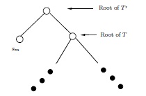

Finally, to see that each \(T' \in {\cal F}_m\) is one of the \(2m-3\) partially labeled trees generated from one and only one \(T \in {\cal F}_{m-1}\), note that by locating the leaf labeled \(s_m\) in \(T'\) one can easily obtain the \(T\) that \(T'\) came from.

Following this triumph the third author half-jokingly suggested that there might be planets on which speciation is \(n\)-ary for some \(n > 2\), and that the counterpart of Professor Dawkins on such a planet would therefore wish to know how many different full \(n\)-ary trees with labeled leafs there are, for each value of the leaf number. (At the time we had not grasped that the Earth's Professor Dawkins was interested iin order-of-descent trees, not pure family trees.) Since the leaf number for such a tree is \(m = k(n-1) + 1\), where \(k\) is the number of non-leafs, it seemed practical to pose the problem in terms of \(k\), rather than \(m\), which is not as freely choosable. We define \(g_n(k)\) to be the number of different (isomorphism classes of) full \(n\)-ary trees with \(k\) non-leafs, with labeled leafs, \(k = 1, 2, \dots\). When \(n = 2\), \(m = k + 1\), and so \[ g_2(k) = f(k+1) = 1 \cdot 3 \cdots (2k-1).\]

Amazingly, based on some (increasingly difficult) computations and inspired guesswork, the gang of four REU participants working on the problem very quickly came up with a proposed recursion formula for \(g_n(k)\):

(1) \[g_n(k) = \binom {nk-1}{n-1} g_n(k-1)\] If valid, this recursion wold determine \(g_n(k)\) for all \(n \geq 2\), \(k \geq 1\), because \(g_n(1) = 1\) for all \(n \geq 1\).

It is straightforward to see that (1) holds when \(n = 2\). It was also found to hold for several small values of \(k\) when \(n \in \{3, 4\}\), and for \(k = 2, 3\) for all values of \(n\). Strong evidence! But the proof in the case \(n = 2\) did not generalize in any way that we could see to give (1).

The second author, with the assistance of the first, refused to give up, and in October or November of 2010, like an archaeologist uncoverng a key relic at an excavation, she ran across a nineteenth century theorem, a graph theory classic with which, as with many classics, we are insufficiently acquainted, which, she saw, would cleanly dispatch the question of \(g_n(k)\).

Cayley's Theorem (West, 2001, Corollary 2.2.4, p. 83)

Suppose that \(t \geq 2\) and \(d_1, \dots, d_t\) are positive integers that add up to \(2t-2\). The number of different trees on labeled vertices \(v_1, \dots, v_t\) in which \(v_i\) has degree \(d_i\), \(i = 1, \dots, t\), is given by the multionomial coefficient \[ \binom {t-2}{d_1 - 1, \dots, d_t -1} = \frac{(t-2)!}{\Pi _{i=1}^t (d_i -1)!}\]

As a corollary one obtains a better-known result, Cayley's Formula: the number of different trees on labeled vertices \(v_1, \dots, v_t\) is \(t^{t-2}\).

Cayley's proof of his theorem, which appeared in 1889, was algebraic, involving generating functions. The proof in (West, 2001) is more combinatorial and graph theoretic, involving Prüfer sequences.

Theorem 2 For \(n \geq 2\), \(k \geq 1\), \[g_n(k) = \frac {(nk - 1)!}{(k-1)!(n-1)!(n!)^{k-1}}.\]

Proof: A full \(n\)-ary tree with \(k\) non-leafs (including the root) has 1 vertex of degree \(n\), \(k-1\) of degree \(n + 1\), and the rest, \(k(n-1) + 1\) of them, of degree \(1\). By Cayley's Theorem, with \(t = nk + 1\), there are \(\frac {(nk-1)!}{(n-1)!(n!)^{k-1}}\) such trees with fully labeled vertices, with the vertices having these prescribed degrees. To count the isomorphism classes of full \(n\)-ary trees with labeled leafs and \(k\) non-leafs, one divides that number by \((k-1)!\), because you get the same leaf-labeled tree for every permutation of the labels among the \(k-1\) vertices of degree \(n+1\).

What remains? As indicated previously, it would be nice to enumerate possible orders of descent of a given cohort of \(m\) terminal species, under the assumption of \(n\)-ary speciation, \(n > 2\). By previous remarks about the trees to which these orders of descent correspond, and Cayley's Theorem, we have a ``formula'' for these numbers, involving a daunting sum of daunting multinomial coefficients. This expression is not totally useless, but it is ugly. Is there a simplification?

Also, it would be of interest to find a proof of Theorem 2 of the same ilk as that of Theorem 1.

Acknowledgements

This work was supported by NSF grant no. 1004933.

References

• Dawkins, R. (1996). The Blind Watchmaker. W. W. Norton & Co., New York.
• West, D. B. (2001). Introduction to Graph Theory. Prentice-Hall, Upper Saddle River, New Jersey, 2nd edition.